Accelerating computations with field-line mapping
This examples highlights some ways to accelerate your calculations with field line mapping. We will use a W7-X case.
import fusionsc as fsc
from fusionsc.devices import w7x
import numpy as np
import matplotlib.pyplot as plt
grid = w7x.defaultGrid()
grid.nPhi = 32
print(grid)
rMin: 4
rMax: 7
zMin: -1.5
zMax: 1.5
nSym: 5
nR: 128
nZ: 128
nPhi: 32
Note: There are two functions to perform axis-current computations, the fsc.flt.axisCurrent and the fsc.devices.w7x.axisCurrent function. They take exactly the same arguments, but fsc.flt.axisCurrent has default behavior tailored towards generic devices, while fsc.devices.w7x.axisCurrent has default parameters more suited for Wendelstein 7-X calculations (current direction, default grid, starting points).
field = w7x.standard()
#field = field + w7x.axisCurrent(field, 2000, grid = grid)

# Note: The above is equivalent to
# field = field + fsc.flt.axisCurrent(field, 10000, grid = w7x.defaultGrid, direction = "cw", startingPoint = [6, 0, 0])

field = field.compute(grid)
Preparing the mapping
To prepare the mapping, we need to (in principle) specify the planes in which we want the remapping to occur. For W7-X, a function with recommended defaults is provided in the w7x device-specific module (same arguments, but different default values).
mapping = w7x.computeMapping(field, toroidalSymmetry = 5)

# Note: The above is equivalent to
# mapping = fsc.flt.computeMapping(
#    field,
#    mappingPlanes = [0],
#    r = np.linspace(4, 7, 200),
#    z = np.linspace(-1.5, 1.5, 200),
#    stepSize = 0.01,
#    distanceLimit = 7 * 2 * np.pi / 8,
#    toroidalSymmetry = 5
# )
geoGrid = w7x.defaultGeometryGrid()
geometry = w7x.op21Geometry().index(geoGrid)
geoMapping = mapping.mapGeometry(geometry.triangulate(0.03), nPhi = 32, nU = 128, nV = 128, toroidalSymmetry = 5)
Inspecting the mapping
After calculating the mapping, we can take a look at the structure of the generated mapping planes. Note: The huge number of NaN values stems from the fact that the corners of the mapping grid extend beyoung the magnetic surface region of W7-X and therefore diverge fast.
data = mapping.download()
lines = str(data).split("\n")

for line in lines:
    if(len(line) > 50):
        line = line[:50] + ' ...'
    print(line)
surfaces: [0]
sections:
  - r:
      shape: [45, 200, 200]
      data: [.nan, .nan, .nan, .nan, .nan, .nan, . ...
    z:
      shape: [45, 200, 200]
      data: [.nan, .nan, .nan, .nan, .nan, .nan, . ...
    traceLen:
      shape: [45, 200, 200]
      data: [.nan, .nan, .nan, .nan, .nan, .nan, . ...
    phiEnd: 1.2566370614359172
    u0: 0.5
    v0: 0.5
    inverse:
      rMin: 3.9961634051526662
      rMax: 7.0066760126216465
      zMin: -1.5066654891827389
      zMax: 1.5067486254418976
      u:
        shape: [45, 200, 200]
        data: [.nan, .nan, .nan, .nan, .nan, .nan, ...
      v:
        shape: [45, 200, 200]
        data: [.nan, .nan, .nan, .nan, .nan, .nan, ...
nPad: 2
nSym: 5
section1 = data.sections[0]
r = np.asarray(section1.r)
z = np.asarray(section1.z)
def plot_grid(x,y, ax=None, **kwargs):
from matplotlib.collections import LineCollection
ax = ax or plt.gca()
segs1 = np.stack((x,y), axis=2)
segs2 = segs1.transpose(1,0,2)
ax.add_collection(LineCollection(segs1, **kwargs))
ax.add_collection(LineCollection(segs2, **kwargs))
ax.autoscale()
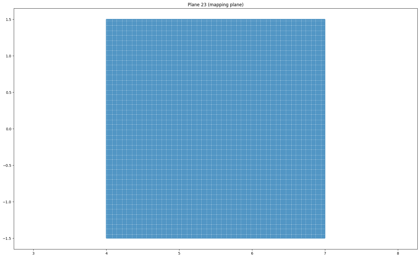
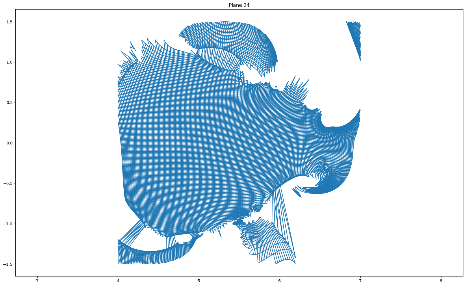
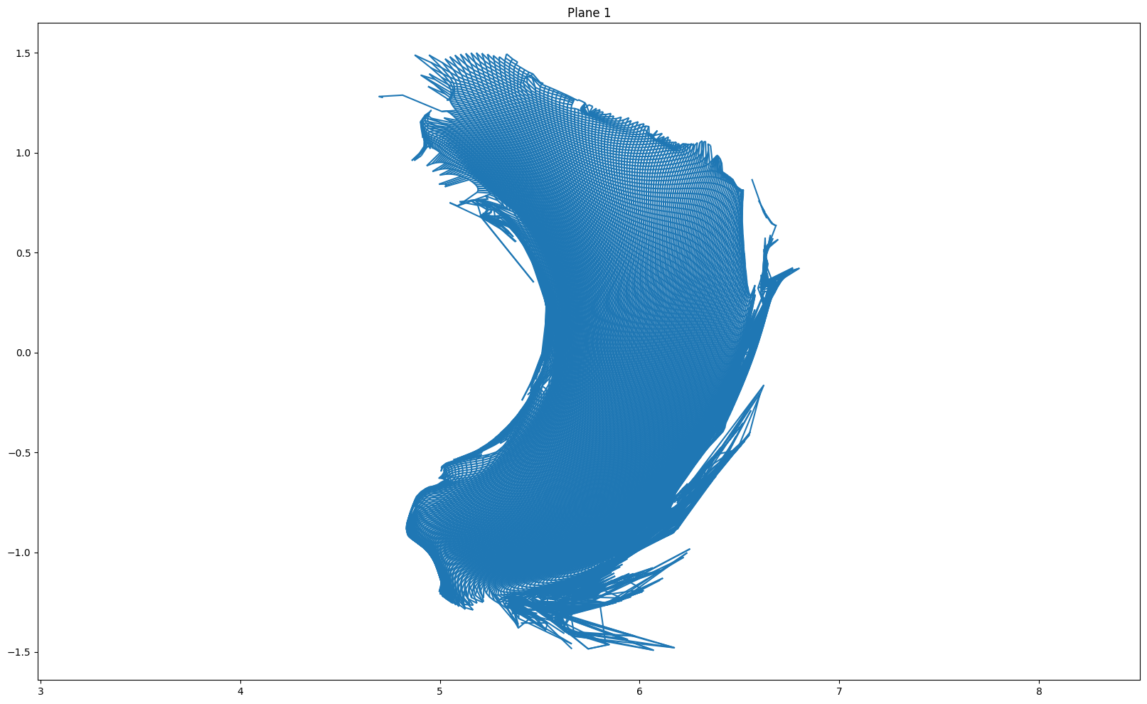
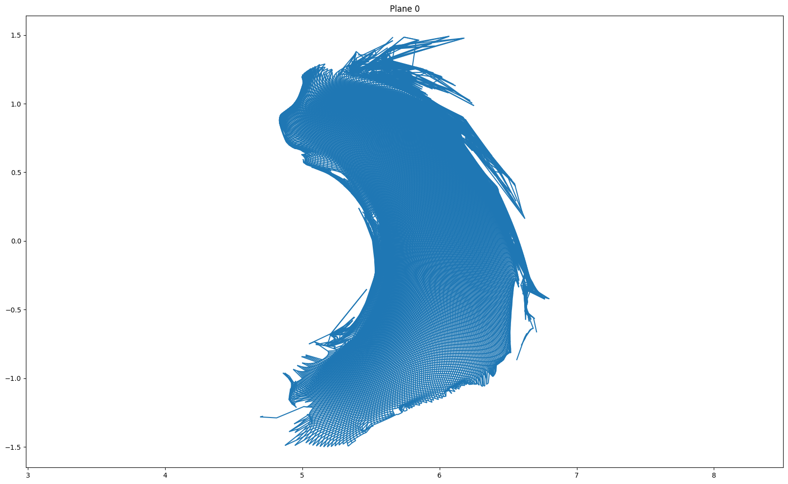
for i in [(len(r) - 1) // 2, (len(r) - 1) // 2 + 1, 0, -1]:
plt.figure(figsize = (20, 12))
plot_grid(r[i], z[i])
plt.axis('equal')
if i == (len(r) - 1) // 2:
plt.title("Plane {} (mapping plane)".format(i+1))
else:
plt.title("Plane {}".format(i + 1))
plt.show()
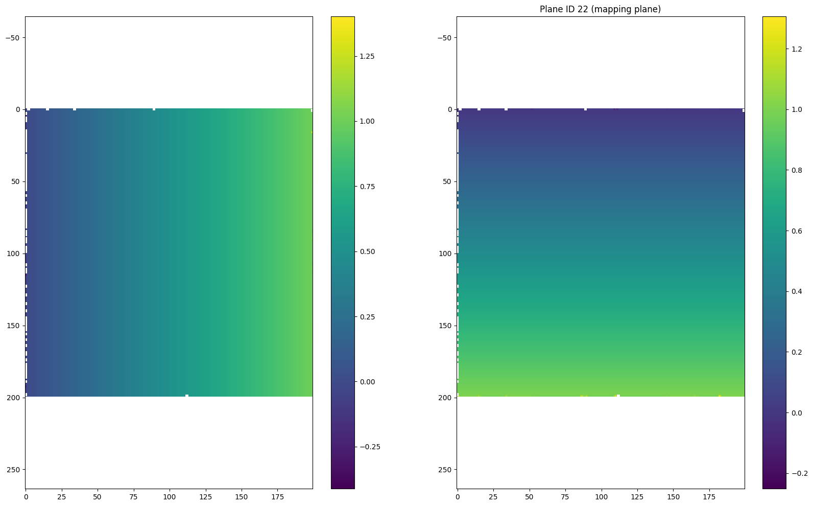
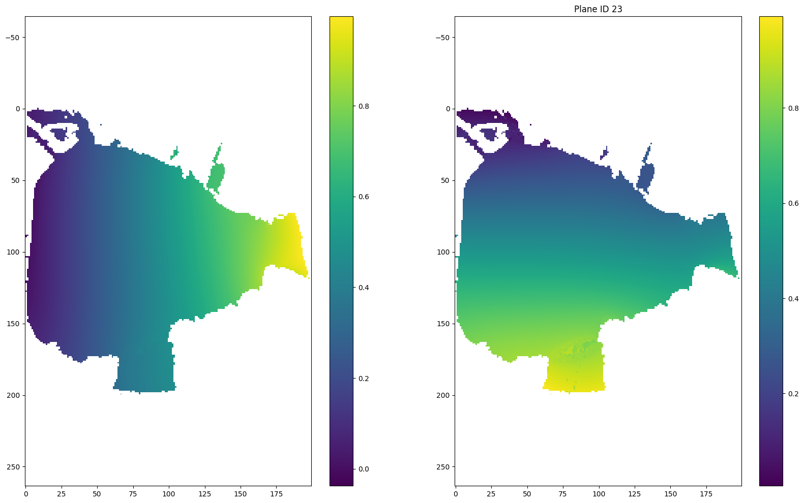
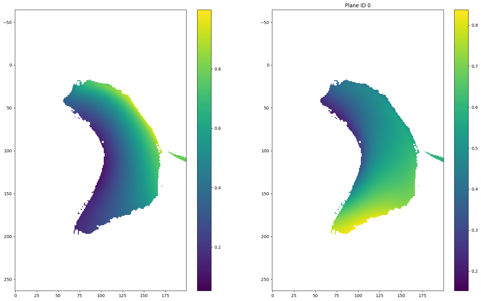
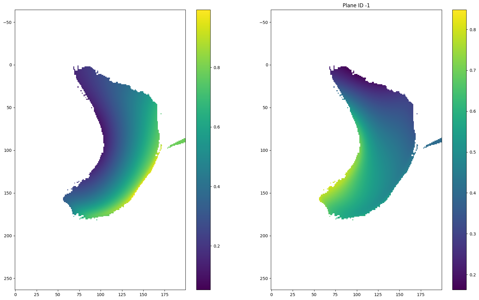
section1 = data.sections[0]

u = np.asarray(section1.inverse.u)# - 0.5
v = np.asarray(section1.inverse.v)# - 0.5

r = np.sqrt((u-0.5)**2 + (v-0.5)**2)
theta = np.arctan2(v-0.5, u-0.5)

for i in [(len(r) - 1) // 2, (len(r) - 1) // 2 + 1, 0, -1]:
    plt.figure(figsize = (20, 12))
    plt.subplot(121)
    plt.imshow(u[i])
    plt.colorbar()
    plt.axis('equal')

    plt.subplot(122)
    plt.imshow(v[i])
    plt.colorbar()
    plt.axis('equal')

    if i == (len(r) - 1) // 2:
        plt.title("Plane ID {} (mapping plane)".format(i))
    else:
        plt.title("Plane ID {}".format(i))
    plt.show()
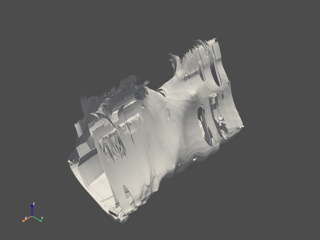
Let’s have a look what the geometry that got translated into field-line coordinate space looks like.
geoMapping.getSection(0).asPyvista().plot(jupyter_backend = "static")
Employing the mapping to accelerate computations
Poincare maps with high turn counts
rStart = np.linspace(4.4, 4.7, 20)
phi = np.radians(72 * 0 + 36)
xStart = np.cos(phi) * rStart
yStart = np.sin(phi) * rStart
zStart = 0 * rStart

pStart = [xStart, yStart, zStart]
#xStart = np.linspace([5.5, 0, 0], [5.8, 0, 0], 40, axis = 1)

pc = fsc.flt.poincareInPhiPlanes(pStart, field, [0, np.pi, np.radians(200.8)], 2000, distanceLimit = 1e7, stepSize = 13, mapping = geoMapping, geometry = geometry)
fsc.flt.trace(pStart, field, turnLimit = 10, stepSize = 0.25, mapping = mapping)
{'endPoints': array([[            nan,             nan,  3.50666860e+00,
          3.53382769e+00,  3.66317276e+00,  4.29309156e+00,
          4.84894922e+00,  4.85245282e+00,  3.67946908e+00,
          3.66018429e+00,  3.66449440e+00,  3.61698542e+00,
          3.60734262e+00,  3.59279260e+00,  3.70441472e+00,
          4.23972572e+00,  4.60137545e+00,  4.62596600e+00,
          4.40231399e+00,  4.25069815e+00],
        [            nan,             nan,  2.67656661e+00,
          2.72258151e+00,  2.93659464e+00,  3.13883633e+00,
          3.65460052e+00,  3.59608176e+00,  2.81685841e+00,
          2.75852686e+00,  2.72098448e+00,  2.80472941e+00,
          2.84222353e+00,  2.88586468e+00,  2.74811552e+00,
          3.14616266e+00,  3.58792946e+00,  3.65961025e+00,
          3.47451925e+00,  3.16519039e+00],
        [            nan,             nan, -9.80648023e-02,
          1.52510911e-01,  5.36120663e-01,  4.53859564e-01,
          1.73727837e-01, -1.33308105e-01, -1.32290696e-02,
          1.43821965e-01,  4.15576592e-02, -4.84073322e-02,
         -1.03235805e-01, -1.95849852e-01, -2.51308064e-01,
          3.81462025e-01,  1.38671629e-01, -2.57872859e-02,
         -2.28434567e-01, -3.44969887e-01],
        [            nan,             nan,  3.65241453e+02,
          3.63739873e+02,  3.63588381e+02,  3.63304331e+02,
          3.63095407e+02,  3.62573910e+02,  3.62826437e+02,
          3.62683451e+02,  3.62558260e+02,  3.62627691e+02,
          3.62673314e+02,  3.62755905e+02,  3.62622598e+02,
          3.63097560e+02,  3.63201610e+02,  3.63152857e+02,
          3.63088168e+02,  3.63003853e+02]]),
 'poincareHits': array([], shape=(5, 0, 20, 10), dtype=float64),
 'stopReasons': array([nanEncountered, nanEncountered, turnLimit, turnLimit, turnLimit,
        turnLimit, turnLimit, turnLimit, turnLimit, turnLimit, turnLimit,
        turnLimit, turnLimit, turnLimit, turnLimit, turnLimit, turnLimit,
        turnLimit, turnLimit, turnLimit], dtype=object),
 'fieldLines': array([], shape=(3, 20, 0), dtype=float64),
 'fieldStrengths': array([], shape=(20, 0), dtype=float64),
 'endTags': {},
 'numSteps': array([ 639,  885, 1365, 1368, 1371, 1372, 1373, 1372, 1378, 1378, 1377,
        1377, 1377, 1377, 1376, 1382, 1383, 1383, 1383, 1383], dtype=uint64),
 'responseSize': 1184}
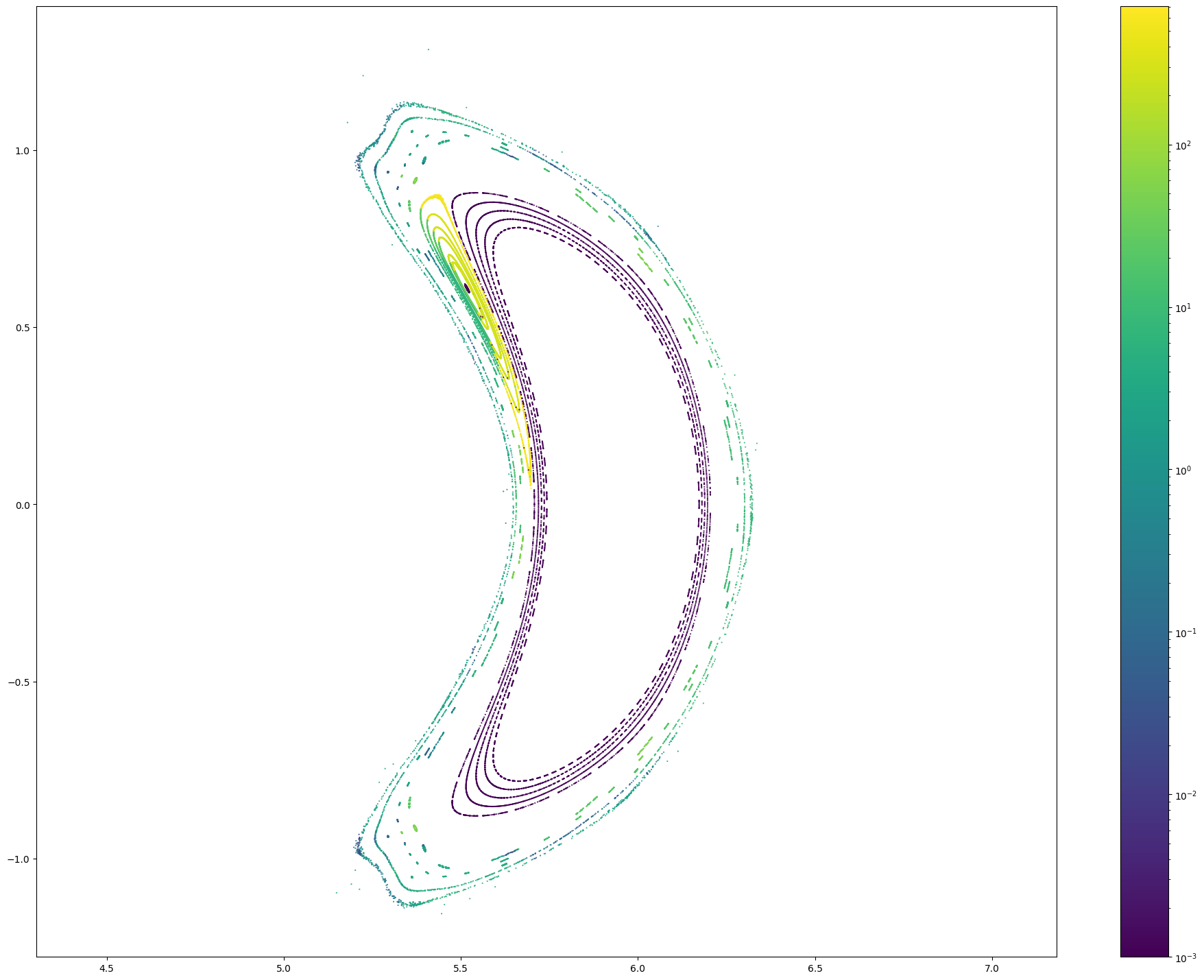
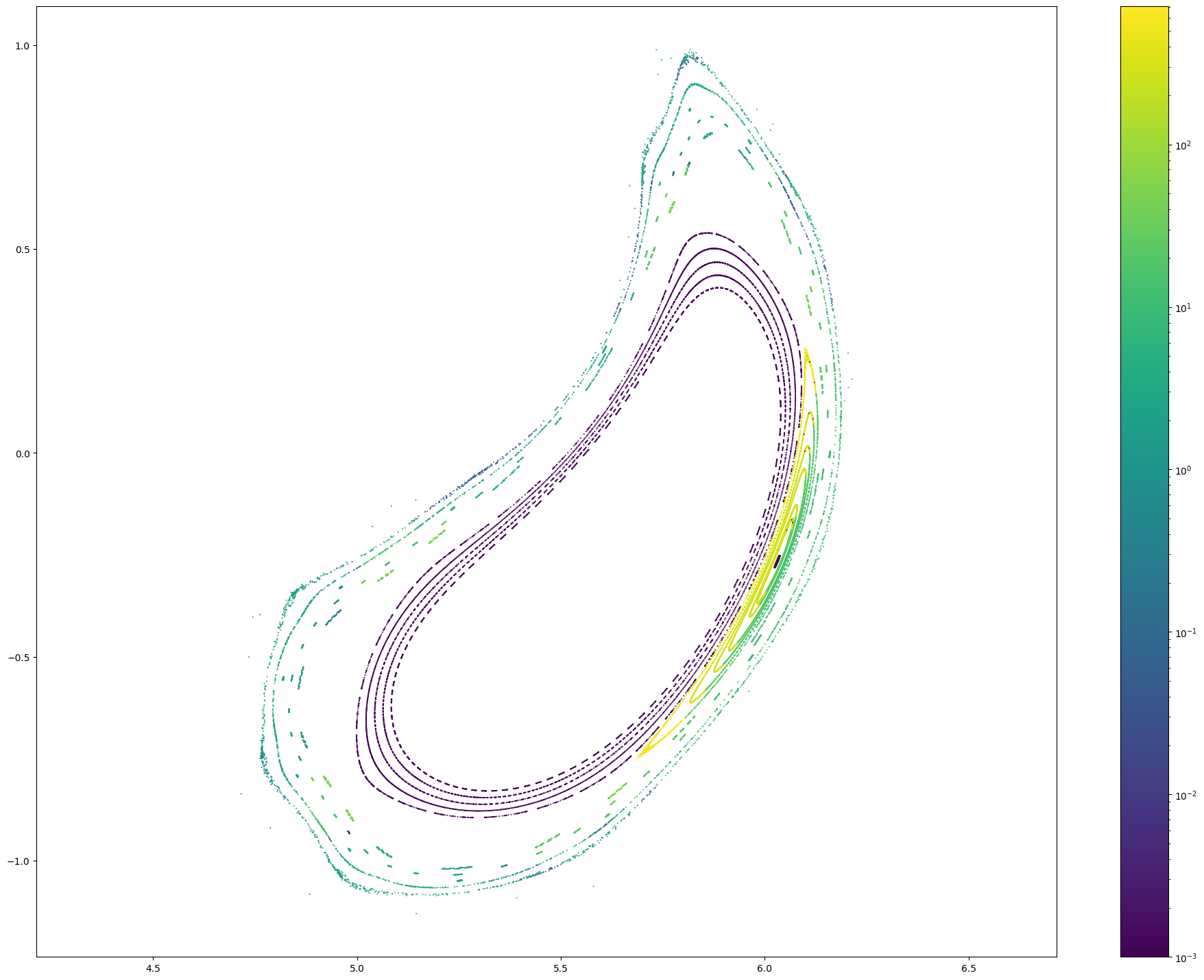
# Let's count the number of Poincare points
np.isfinite(pc[0]).sum()
102088
from matplotlib.colors import LogNorm

x, y, z, lF, lB = pc
r = np.sqrt(x**2 + y**2)

for i in range(len(x)):
    plt.figure(figsize = (24, 18))
    plt.scatter(r[i], z[i], c = np.maximum(lF + lB, 0.001)[i], marker = '.', s = 1, norm = LogNorm())
    plt.colorbar()
    plt.axis('equal')
#plt.xlim(4.5, 4.75)
#plt.ylim(-0.4, 0.4lB
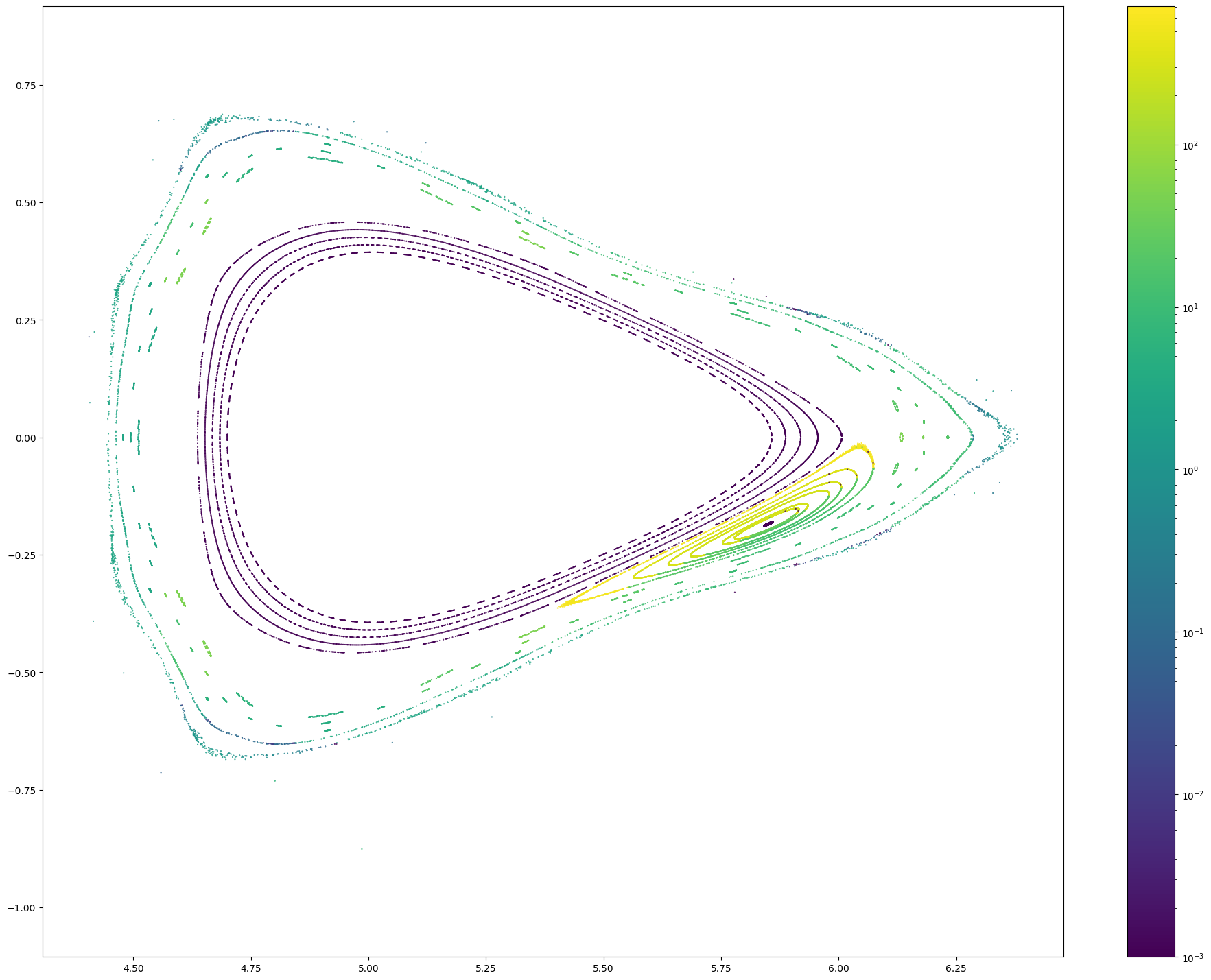
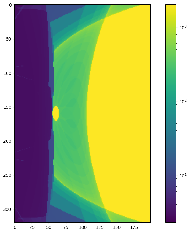
High-resolution connection length distributions
from fusionsc import backends

r = np.linspace(4.5, 4.75, 200)
z = np.linspace(-0.4, 0.4, 320)

rg, zg = np.meshgrid(r, z, indexing = 'ij')
xg = -rg
yg = 0 * rg

def calc_len(d):
    return fsc.flt.connectionLength([xg, yg, zg], field, geometry, mapping = geoMapping, distanceLimit = 1e3, stepSize = 13, direction = d)

import time
start = time.time()
lc = calc_len('forward') + calc_len('backward')
end = time.time()
print(end - start)
32.38329029083252
from matplotlib.colors import LogNorm
plt.figure(figsize = (12, 9))
plt.imshow(lc.T, norm = LogNorm())
plt.colorbar()
<matplotlib.colorbar.Colorbar at 0x1f709656890>
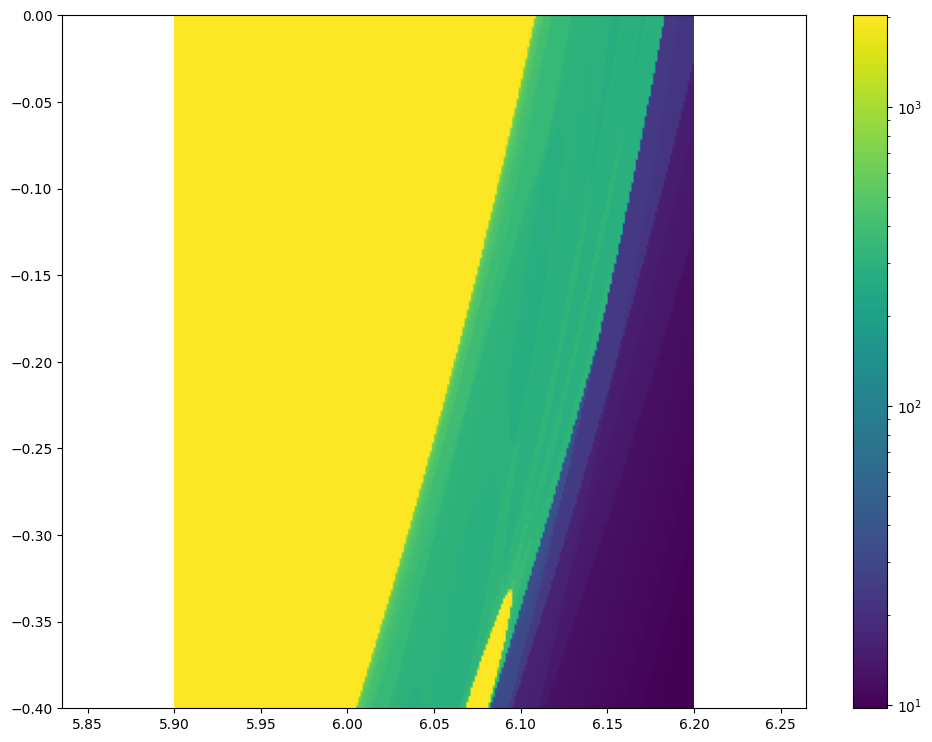
r = np.linspace(5.95, 6.1, 240)
z = np.linspace(-0.25, -0.1, 240)
phi = np.radians(200.8)

rg, zg = np.meshgrid(r, z, indexing = 'ij')
xg = np.cos(phi) * rg
yg = np.sin(phi) * rg

def calc_len(d):
    return fsc.flt.connectionLength([xg, yg, zg], field, geometry, grid = grid, mapping = geoMapping, distanceLimit = 1e3, stepSize = 13, direction = d)

import time
start = time.time()
lc = calc_len('cw') + calc_len('ccw')
end = time.time()
print(end - start)
33.065414905548096
from matplotlib.colors import LogNorm
plt.figure(figsize = (12, 9))
plt.imshow(lc.T, norm = LogNorm(), origin = "lower", extent = [5.9, 6.2, -0.4, 0])
plt.colorbar()
plt.axis('equal')
(5.9, 6.2, -0.4, 0.0)